Python – LLM Quantization with Qwen3

Quantization is one of the most common techniques to make language models smaller and more practical. The idea is simple – instead of storing model weights with high numerical precision, these are replaced with lower precision approximations. This reduces the amount of information each weight can carry and that can affect the quality of the model.

In this article, it is tested how quantization changes the behavior of small language model on a set of simple tasks. The results are smehow expected. At higher precision, the model behaves as expected and at lower precision, its preferences go into random.

The first image shows the basic mechanics of quantization on a single number, -0.41 is picked using 8-bit symmetric quantization with round-to-nearest integer.

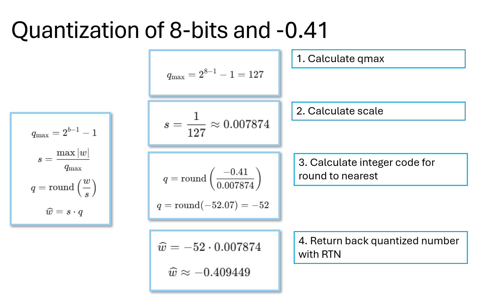
The steps are explicit and you see yourself how -0.41 is transfered to -0.409449. The difference is approximately 0.000551, so the original value is perserved quite closely in the example. However, using fewer bits means having fewer available values on the quantization grid. The approximation can then become rough. The next image applies teh same method to a larger set of example numbers:

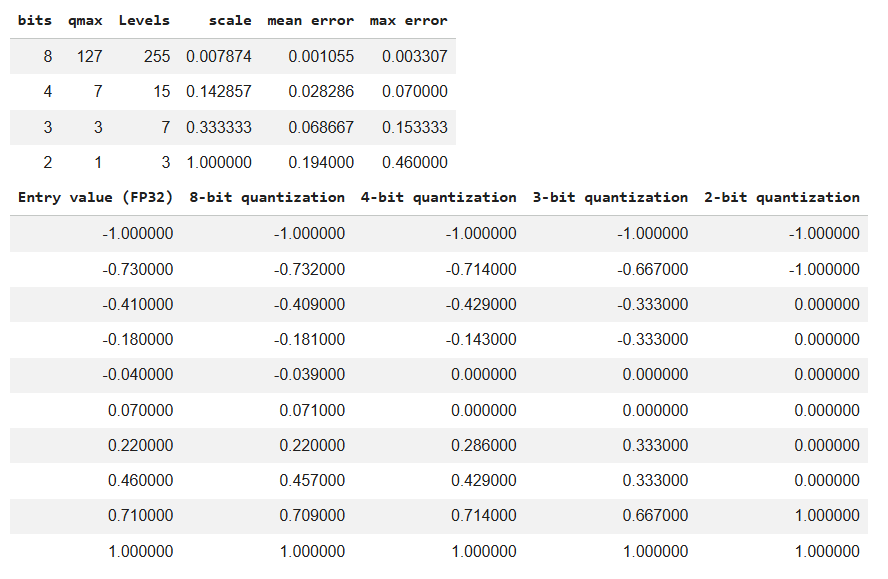
You see that 0.46 becomes 0.457 -> 0.429 -> 0.333 -> 0. The question is what happens when we apply these approximations to model weights rathan than just presenting it in a table. Before testing the results, we need to clarify what we are quantizing in Qwen 3 and what we are leaving unchanged.

What are we quantizing?

We apply quantization to two groups of linear weight matrices inside Qwen3-0.6B-Base.

• Attention weights: q_proj, k_proj, v_proj, and o_proj. These help determine which information the model attends to and how the attention results are combined.
• MLP (Multi-layer perceptron) weights: gate_proj, up_proj, and down_proj. These transform the information inside each Transformer block and account for a large share of the model parameters

Together, these groups contain 196 weight matrices with approximately 440.4 million weights, out of 596 million parameters in the complete model. In other words, we are applying quantization to approximately 74% of the model parameters, not to the entire model.

What are we not quantizing?

• embeddings, which convert token IDs into initial vectors
• output head, lm_head, which converts the final representation into scores for the tokens in the vocabulary
• normalization parameters and bias parameters. Normalization helps maintain stable activation scales, and biases add offsets to layer outputs.

These parameter groups are small compared with the weight matrices being quantized.

So, when we refer to the 4-bit configuration, we mean that the selected attention and MLP weights have been approximated using 4-bit quantization grid. We do not mean that every parameter has been converted to 4 bits. There is one more practical detail: the notebook, following the article reconstructs the rounded weights and stores these as floating point tensors, as we are testing how lower-precision approximations affect answer quality and not measuring memory savings or faster executions. With these points, let’s move from rounding numbers to seeing whether the model still ranks the correct answers first and when does it stop doing so.

In the attached jupyter notebook file, we have decided to ask Qwen3 to answer 10 simple closed questions with 4 answers each:

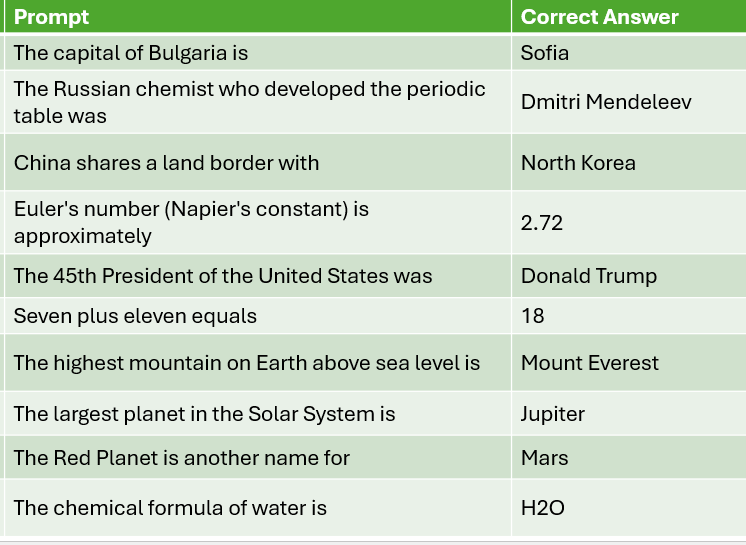
Does the model still rank the correct answer first?

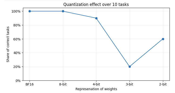
With 16bits (original) that might seem naive and simple, as the model is actually good at answering (it is currently 2026 outside, not 2019), but as we start reducing the bits, some interesting results start showing up:

Once again, there is an important detail of the test –  the model does not generate answers freely, but evaluates each candidate as a continuation of the prompt and calculates the average log-probability of its tokens. The candidate with the highest average is ranked first.

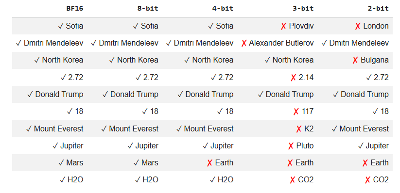
In these results, we see that original model and 8-bit configuration both achieve the 10/10 score. At 4-bit we have 1 wrong answer and at 3-bits it falls to 2/10, before recovering to 6/10 at 2 bits. With four candidates and one correct answer per task, uniform random guessing would achieve 25% accuracy on average. Thus, the 3-bit result is below the average, but ten tasks are not enough to conclude that the model is generally worse than random guessing. The recovery at 2 bits is also worth noticing. Reducing the precision does not produce a steady decline in the number of correct answers. This does not establish that 2-bit quantization is better than 3-bit quantization. but it simply shows what happened with this specific method, prompts and candidate answers.

Changing the selected capital of Bulgaria from Sofia to Plovdiv to London

Let’s zoom a bit on the first task, finishing the prompt “The capital of Bulgaria is…” and seeing the candidates – [Sofia, Veliko Tarnovo, Plovdiv, London]:

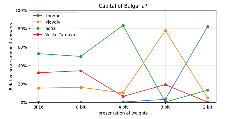
For the original model, Sofia receives approximately 52.7% of the relative score among the candidates. At 8 bits, that score becomes 49.7%, but it still ranks first. At 4 bits, its relative score increases to 83.5%, leaving the sum of the other 3 to be below 27%. At 3 bits, the ranking changes completely and Plovdiv takes the first place with 77.7%, while Sofia falls to the last place. At 2 bits, London takes first place with approximately 81.9%.

Thus, the lower precision configuarations are not merely giving the correct answer a slightly lower score – they are placing incorrect candidates first, by a large margin.

What do these percentages mean?

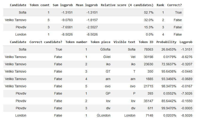
For this prompt and tokenizer, Sofia and London, each occupy one candidate token. Plovdiv occupies three [P-lov-div], while Veliko Tarnovo is split into five – [Vel-iko-T-arn-ovo]. The notebook first calculates the mean log probability for each candidate.

mean_logprob = sum_logprob / token_count

It then applies softmax to the four mean log-probabilities, producing relative scores that sum to 100%. A higher mean log-probability produces a higher relative score.

Sofia receives 52.7%, which is more than the other three candidates combines. This is not a 52.7% probability that “Sofia” is the correct answer. It is a relative score calculated from tehse four candidates using this particular scoring method. That also explains why Sofia has a different percentage in the token-level table. Its token has a probability of approximately 26.8% after the prompt. The 52.7% figure comes from comparing its score with those of the other three candidates.

Why Veliko Tarnovo has 98.3473% probability, but is not selected?

That is a good question and if you are looking at the table above you might be puzzled. What can be higher than that? The answer is that finishing an answer is not the same as choosing it. And the 98.3473% is actually the probability for the final token ovo. With other words, after the supplied text:

The capital of Bulgaria is Veliko Tarn

the model assigns the probability to ovo as the next token, completing the name of the city. The score is lower, because the first token of the candidate, Vel, receives only 0.0179%. And that low initial probability pulls down the score, even though the remaining pieces are much more likely once the name has started. But to evaluate an answer, we should take a look at all its tokens, and for Veliko Tarnovo the sum is -9.0783. That, divided by 5 gives a mean log-probability of -1.8157 and the one from Sofia is actually way better -1.3151. So, the model can be very good at completing an incorrect answer (98.3%), but what matters is all the tokens and their average.

What this experiment shows?

First of all, it shows that it is actually extremely cheap to “play” with models and tokenization. As far as you have interest you can easily do it and look for some results and how to interpret them. You might say that on these ten tasks, the 8-bit configuration preserves all correct first-place answers, while the 4-bit conguration loses one. At lower precision configurations, the ranking changes dramatically. However, these results describe a small candidate ranking experiment, not a general benchmark of everything a model can do. The sample is tested just once (with fixed random, of course) and the results can actually vary with bigger sample. My idea was to show, that quantization is doable and not a science fiction with extreme needs of hardware. If that task sparkled some interest in you, consider changing the questions, and increasing them, into seeing how a model “breaks” and where “exactly”. 🙂

Of course, the code is available here – https://github.com/Vitosh/Python_personal/tree/master/PythonProjects/LLM-Quantization-Qwen3

Enjoy the day and smile more 🌵🐻😄.